Title : Exponential Growth, Exponential Decay, and Goal Seeking Behavior

|
Location : Home > Methods > Simulation > System Dynamics > Introduction to System Dynamics Title : Exponential Growth, Exponential Decay, and Goal Seeking Behavior |
 |
Exponential Growth, Exponential Decay, and Goal Seeking Behavior
�@���̃Z�N�V�����ł͂R�̊�{�I�U�镑���̃��[�h�ł���w���I�����E�w���I�����E�ڕW�T���̃_�C�i�~�b�N�������������̎��Ԍo�H��͕킵�A�P���ȃV�X�e���_�C�i�~�N�X�̍\���𗝉�����Ӑ}�������Ċm�F����B�O�͂ŐG�ꂽ�\�z�u���b�N��p���A���߂ēǎ҂ɃV�X�e���_�C�i�~�N�X�̃R���s���[�^�V�~�����[�V�������f�����Љ��B���������̑O�ɉ�͓I�ȉ�@�ƃV�~�����[�V�����ɂ���@�̈Ⴂ�������Ă����K�v�����낤�B
Analytical Versus Simulated Solutions
�@Chapter 3 �ŋL�����X�g�b�N�̓�����z�N���Ă��炢�����B���Ȃ킿�X�g�b�N�͋L�^���A�t���[�̎��Ԍ`��itime shape�j��ω������A�t���[�f���A�x��idelays�j�ݏo���B���āA��̓I�ɃR���s���[�^���ǂ̂悤�ɃX�g�b�N�E�t���[�\���̐U�镑�����v�Z���邩���������Ă݂悤�B�P���Ȑ��^�t�B�[�h�o�b�N�V�X�e���Ɋւ���c�_���đ����̃X�g�b�N������A���̊Ԃ́i���X�ɂ��Ĕ���`�́j���ݍ�p�ɂ��Ή�����t���[�����G�Ŏ��ԂƂƂ��ɘA���I�ɕω�����ɓ��ݍ��ނɂ�A�R���s���[�^�V�~�����[�V�����̑�ނ͏d�v�ɂȂ��Ă���B����������A���̖��͐l�Ԃ̔F�m���E�ɒB���ăV�X�e���̃_�C�i�~�b�N���𖾂炩�ɂ��邽�߂ɃR���s���[�^�V�~�����[�V�������K�v�ɂȂ����Ƃ��ɏ��߂ďd�v�ɂȂ�B

�}�P�F�X�g�b�N�ƃt���[�̗�
�@��̐}�P�� Chapter 3�iStocks and Flows �Z�N�V�����̐}�P�j�ōŏ��Ɏ������}�̍Čf�ł���B Given this structure, Figure 2 below shows the time path of the flow which, in this instance, is linear and set at an arbitrarily determined constant positive value. In other words, the flow valve is opened to some positive value and does not change from this position over ti
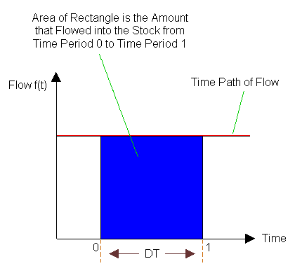
�}�Q�F�X�g�b�N�ւ̗����ʂ������`�̖ʐ� (DT = 1)
Knowing that flows cause stocks to fill or drain, looking at the time path of the flow variable in Figure 1 we can say that the height to which the stock will fill due to its rate of flow over the (arbitrarily determined) time period from t=0 to t=1, is the area beneath the time path of the flow from period t=0 to t=1. This is shown by the shaded rectangle in Figure 2. The area of the rectangle is easy to calculate, of course, as it is merely the height of the rectangle (i.e., the value of the flow at any point from t=0 to t=1) multiplied by the length of the rectangle (i.e., the time span from t=0 to t=1). If we define the time span from t=0 to t=1 to be "DT" then the:
|
�m���� 0 �Ǝ��� 1 �̊Ԃ̃X�g�b�N�ւ̗����ʁn ���m�����`�̖ʐρn ���m�t���[�̒l�n�~�m���Ԃ̕ω��ʁn �� f(1) * DT ���P
|
Simulated Solutions
The situation gets a little more complicated, however, when the flow variable in Figure 1 is not constant but changes over time. Figure 3 is a graph of a quadratic inflow to the stock (i.e., one that is nonlinear with one "bend" or "curve"). Applying the same logic that was used in the last example -- i.e., finding the area of a rectangle "beneath" the time path of the flow -- yields an overestimate of the amount that has flowed into the stock from t=0 to t=1. The "wedge" area above the curve in Figure 3 is the amount by which the rectangle overestimates the amount that has flowed into the stock.
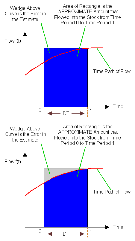
Figure 3: The Approximate Amount that Flowed into the Stock is the Area of the Rectangle (DT = 1)
But what if the change in time, DT, is made smaller? What if DT is, say, cut in half? Figure 4 replicates the time path from Figure 3, but shows a DT of .5 -- i.e., half as large as before.
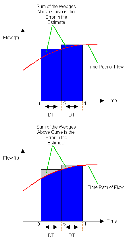
Figure 4: Approximating the Amount that Flowed into the Stock (DT = .5)
Analytical Solutions
In principle, a dynamical system�fs time step, DT, could be cut in half forever. If this were to occur, the error in approximating the amount that flowed into the system�fs stocks would be systematically reduced until it became infinitesimally small. In more traditional mathematical notion this means that the:
|
Exact Amount that Flowed into Stock from Time Period 0 to Time Period 1 = lim DT -> 0 [ t=0��t=1f(t) * DT ] = t=0��t=1 f(t) * dt Equation 5
|
Equation 5 represents (in general terms) the continuous time version of the dynamical system presented in Figure 1. In this version of the model, DT is infinitesimally small and the solution to the equation reveals exactly how much has flowed into the system�fs stock from t=0 to t=1. The solution to Equation 5, if it exists, is an exact analytical solution.
In contrast to simulated solutions, analytical solutions are general solutions to dynamic systems of equations. Rather than revealing the approximate amounts that have flowed into a system�fs stocks at short time intervals (DTs) between successive computations, they reveal the exact amounts that have flowed into a system�fs stocks at any period of time. In other words, for any system possessing an analytical solution, any time period can be substituted into the solution and it will yield the exact amounts that have flowed into the system�fs stocks. The solution does not require the calculation of the amounts that flowed into the system�fs stocks in all earlier periods of time. In addition, the form of a system�fs analytical solution reveals much about the general nature of its dynamics, even without any numerical computation.
Given all of the apparent advantages offered by exact analytical solutions, why do modelers bother to use simulated solutions at all? The answer is quite simple: only linear systems have exact analytical solutions. This is because: (1) they can be broken down into parts, (2) the behaviors of the parts can be determined, and (3) the behavior of the entire system can be found by adding together the behaviors of the parts. In other words, the behavior of a linear dynamical system is merely the sum of the behaviors of its parts.
Nonlinear systems, on the other hand, cannot be broken down into pieces and solved analytically. They must be analyzed as a whole. The connections between the parts of a nonlinear system are as vital to its behavior as the pieces themselves. Indeed, the behavior of a nonlinear system is more than merely the sum of the behaviors of its parts. Since nonlinear dynamical systems do not have exact analytical solutions, their behavior can only be determined through simulation.
In sum, if the real world is nonlinear (i.e., has limits), if humans are incapable of thinking through all of the dynamic implications of their mental models, and if nonlinear dynamical models have no analytical solutions, simulation modeling is necessary for improved dynamical thinking and learning.
Exponential Growth
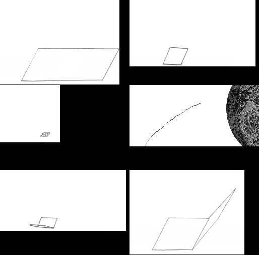 | 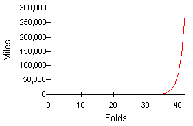 |
| Figure 7a: Folding a Piece of Paper | Figure 7b: Exponential Growth of the Thickness of a Piece of Paper |
In terms of a system dynamics model that can produce exponential growth, consider Figure 8 -- a "first cut" stock-flow structure of an elephant herd system. The figure presents the model�fs stock and flow icons, the corresponding system dynamics equations, and the dimensions of each equation. As will become apparent throughout the remainder of this book, the specification of the dimensions of every equation in a system dynamics model is an important part of the modeling process. It helps the modeler both document a model and conceptualize its structure. Stocks are dimensioned in terms of "units" ("Elephants") and flows are dimensioned in terms of "units/time" ("Elephants/Year"). Other variables in a system dynamics model must possess dimensions that correspond algebraically to its stock-flow-feedback loop structure. Examples of system dynamics models that have been properly dimensioned will be presented ahead.
|
|
Figure 9 presents a simulation of the "first cut" model, when the initial number of elephants in the herd is set at ten and a constant number (two) of baby elephants are born each year. Clearly the model exhibits a linear, rather than an exponential, growth.
(Click on image to run simulation)
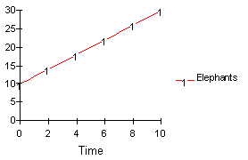
Figure 9: Simulation of the First Cut of the Elephant Herd Model (Initial Elephants = 10)
Before moving directly to a structure that exhibits the exponential time shape, it is perhaps better to "think like a modeler" for the moment. A good system dynamicist will test each of the structures he or she creates for "robustness." This means that he or she will test to see if their model behaves "properly" under a variety of circumstances, both normal and extreme. If a model behaves properly in response to robustness testing, the system dynamicist can be confident that it will behave properly when interfaced with other model structures.
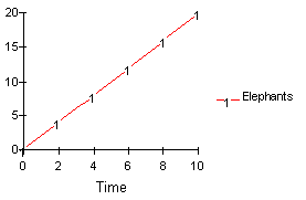
Figure 10: Simulation of the First Cut of the Elephant Herd Model (Initial Elephants = 0)
Figure 10 shows the results of a robustness test done on the "first cut" elephant herd model. For the purpose of the test, the initial number of elephants in the herd (stock variable) was changed to zero. Clearly the simulation makes no sense. The number of elephants in the herd grows even though there are initially no elephants to produce baby elephants. The conclusion is that the model does not behave properly in response to this extreme test and is therefore "nonrobust."
The next cut of the model should be aimed at correcting the robustness problem. The first cut of the model generated an implausible result because elephants are needed to produce more elephants. This biological fact implies that a feedback link from the stock of elephants to the flow of elephant births is required so that the computer can calculate the number of baby elephants produced by the elephant herd each year.
Figure 11 presents the "second cut" of the elephant model. It contains a feedback link from the stock of elephants to the birth rate flow, an additional icon (the birth rate coefficient (BirthRateCoef)), and an additional information link.
|
|
Figure 12 shows the results of a simulation of the model when the initial number of elephants is set at zero. Clearly, the new formulation of the model has cured the robustness problem revealed in Figure 10. When there are initially no elephants in the herd, no baby elephants are born and the size of the herd remains at zero. (click on image to run simulation)
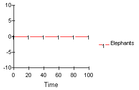
Figure 12: Results of a simulation using "Second Cut" of the Elephant Herd Model (Initial Elephants = 0)
Figure 13, on the other hand, is a simulation of the model when the initial number of elephants is ten. In this case, the positive feedback loop created between elephants and baby elephants causes the exponential growth path of the elephant herd. (Click on image to run simulation)
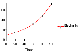
Figure 13: Simulation of the "Second Cut" of the Elephant Herd Model (Initial Elephants = 10)
Generic Structure
Over the years, system dynamicists have identified combinations of stocks, flows and feedback loops that seem to explain the dynamic behavior of many systems. These frequently occuring stock-flow-feedback loop combinations are often referred to as "generic structures".
Figure 14 shows a generic structure responsible for exponential growth and its corresponding causal loop diagram. It is the generic version of Figure 11 -- a generic first order positive feedback loop system. Most system dynamicists think about this structure when modeling a system that grows exponentially; the contents of the stock produces more of the contents of the stock.
|
|
Figures 15 and 16 illustrate two other specific instances of this generic structure. Figure 15 shows positive exponential feedback in an interest compounding savings account. Figure 16 shows how knowledge accumulates in a particular scientific field of study.
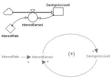
Figure 15: Structure for a simple interest compounding savings account
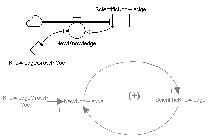
Figure 16: Structure for the growth of knowledge in a particular flield of study
Exact Analytical Solution for a First Order, Linear, Positive Feedback Loop System
The first order positive feedback loop system of Figure 14 is a linear system. As a result, in addition to its simulated solution, it possesses an exact analytical solution. This solution is:
|
Stockt = Stock0 * e Coef * t Equation 1 |
For the more mathematically inclined reader, the derivation of this solution is shown in the box below. Although the case has already been made that simulated solutions to nonlinear systems are preferable to analytical solutions to linear systems, Equation 1 can be used to generate some insights that are useful in system dynamics modeling.
|
Derivation of the Analytical Solution
Therefore, the exact analytical solution is:
Stockt = Stock0 * eCoef * t |
Using the Exact Analytical Solution to Test Numerical Integration Methods
Equation 1 can be used to determine the accuracy of various simulated solutions to the generic first order positive feedback loop system shown in Figure 14. Generally speaking, simulated solutions to system dynamics models differ by step size (DT) and/or numerical integration method employed. As was previously discussed, reducing DT makes a simulated solution more accurate, but forces the computer to do more work. In a similar way, numerical integration methods vary by accuracy and required number of calculations.
Most system dynamics software packages go through the following sequence of events to simulate a model:
|
Initialization Phase
Iteration Phase
|
Step 1 of the Iteration Phase is the place where most numerical integration methods differ. More specifically, different numerical integration methods estimate the change in a model's stocks over the interval DT in different ways. Although many numerical integration methods exist, the two that are most frequently used in system dynamics modeling are Euler's method and a second order Runge-Kutta method. Euler's method is the simplest and least accurate (for a given DT) numerical integration method available. Indeed, due to its conceptual simplicity, it is the method upon which the nomenclature of the generic system dynamics stock equation is based. In Step 1 of the Iteration Phase of the simulation of a system dynamics model, Euler's method estimates the change in a model's stocks over the interval DT as:
DStock = DT * Flow at Beginning of DT
Thus, in Step 2 of the Iteration Phase, the new values for a model's stocks are calculated in the following way:
Stockt = Stock(t-DT) + D Stock
Stockt = Stock(t-DT) + DT * (Flow(t-DT) => t)
Of course, this is precisely the same formulation as Equation 4 of Analytical-vs-Simulated Solutions.
A second-order Runge-Kutta method differs from Euler's method in that it uses two flow calculations within a given DT to create an estimate for the change in a model's stocks over the interval DT. More precisely, during Step 1 of the Iteration Phase of a simulation, a second order Runge-Kutta method estimates the change in a model's stocks over the interval DT as:
F1 = DT * Flow at Beginning of DT [same as in Euler's method]
F2 = DT * Flow at End of DT = DT * Flow(Stock(t) + F1)
D Stock = 1/2 * (F1 + F2)
Stockt = Stock(t-DT) + D Stock
Stockt = Stock(t-DT) + 1/2 * (F1 + F2)
In other words, a second-order Runge-Kutta method estimates the change in a model's stocks by taking the mean of the flows that occur at the beginning and at the end of each time step.

Figure 17: Comparison of Exact Analytical Solution to Simulated Solution (Euler's Method; DT = .5)
Figure 17 compares the results of simulating the generic first order positive feedback loop system shown in Figure 14 via Euler's method with a DT of .5, against the exact analytical solution to the system given by Equation 1. In each case, the initial value of the stock is set equal to 100 units and the value of the growth coefficient is set at .02 units/unit/time. Athough each solution starts at the same place, the simulated solution quickly diverges from its exact counterpart. Indeed by period 10, the exact amount in the stock is 122.14 units, while the simulated solution indicates that it contains only 122.02 units. In a similar way, Figure 18 compares the exact analytical solution to the generic first order positive feedback loop system against a simulated solution using Euler's method and a DT of .25. Clearly, cutting DT in half improves the accuracy of the simulated solution, as the simulated value of the stock at period 10 is now 122.08.
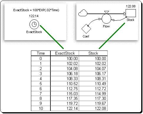
Figure 18: Comparison of Exact Analytical Solution to Simulated Solution (Euler's Method; DT = .25)
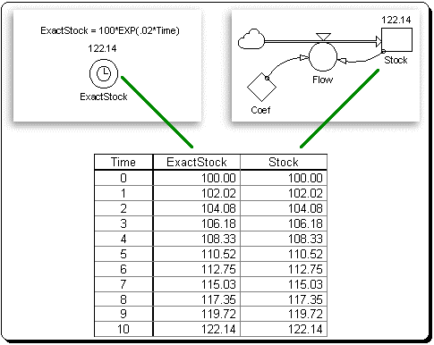
Figure 19: Comparison of Exact Analytical Solution to Simulated Solution (Second Order Runge Kutta Method; DT = .25)
Measures of Exponential Growth
The exact analytical solution to a first order, linear, positive feedback system (Equation 1) can be used to derive two important measures of exponential growth. The first of these measures is the system's time constant. The second is sytem's doubling time.
Time Constant
Figure 20 depicts a system dynamics representation of a first order, linear, positive feedback loop system with an exact analytical solution represented by Equation 1. The time constant of this system, Tc, measured in units of time, is defined to be 1/Coef.
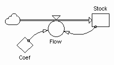
Figure 20: First Order, Linear, Positive Feedback Loop System
Given the definition of the system time constant, the following question can be asked: How much exponential growth occurs during one time constant's worth of time? To answer this question, the system's time constant must be inserted into equation 1. Thus, the amount of exponential growth that occurs during one time constant of time is:
Stockt = Stock0 * eCoef * t
Stockt = Stock0 * eCoef * Tc
Stockt = Stock0 * eCoef * (1/Coef)
Stockt = Stock0 * e1
Stockt = Stock0 * 2.71828
In other words, the amount of exponential growth that occurs during one time constant is 2.71828 times the initial amount in the system's stock. Pushing this logic to the next step, the amount of exponential growth that occurs during two time constants is 7.3890 (i.e., 2.71828 * 2.71828) times the initial amount in the system's stock.
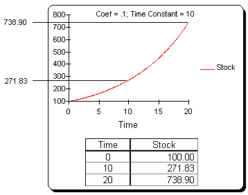
Figure 21: Exponential Growth After One and Two Time Constants have Elapsed
Figure 21 shows the amount of exponential growth that has taken place in a first order, linear, positive feedback loop system, with a Coef of .1 and an initial value of 100, after one and two time constants have elapsed. After one constant, the stock has grown from 100 to 271.83 and after two time constants it has grown to a value of 738.90.
Doubling Time
The second measure of how quickly exponential growth is proceeding in a first order, linear, positive feedback system is its doubling time. A system's doubling time is simply the amount of time it takes for the contents of its stock to double. The doubling time of a first order, linear, positive feeback loop system, Td, is equal to seventy percent of its time constant. That is: Td = .7 * Tc . For the more mathematically inclined reader, the derivation of this result is provided in the shaded box below.
Derivation of the Doubling Time for a First Order, Linear, Positive Feedback Loop System |
| The doubling time for a first order, linear, positive feeback loop system is calculated using Equation 1. If the doubling time, Td, is defined to be the time it takes to double the initial value of a stock, then:
2*Stock0 = Stock0 * eCoef * Td Since the system's time constant, Tc, is 1/Coef, then the system's Coef = 1/Tc. Thus:
2 * Stock0 = Stock0 * e1/Tc * Td Dividing both sides by Stock0 yields:
2 = eTd/ Tc
ln(2) = ln(eTd/ Tc) �܂���
.69 = Td/ Tc �܂���
.7 = Td/ Tc �܂���
Td = .7 * Tc Thus, the doubling time of a first order, linear, positive feeback loop system is seventy percent of its time constant. |
Figure 22 shows the same simulation run presented in Figure 21. This time the figure shows that the system's stock doubles from a value of 100 to a value of 200 in (approximately) the seventh period (.7 multiplied by the time constant of 10 periods).
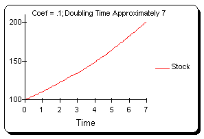
Figure 22: Doubling Time for a First Order, Linear, Positive Feedback Loop System
The concept of doubling time leads directly to a heuristic known as the Rule of 70. This rule says that, if you know, or can estimate, how quickly an exponentially growing system is growing (i.e., if you know, or can estimate, Coef in Equation 1), you can calculate its doubling time as Td = (70 / Coef) * 100.
Consider, for example, the growth of the United States economy. As shown in Figure 23, U.S. nominal GDP grew exponentially at a rate of 7 percent per year, from 1959 to 1995 (i.e., Coef is estimated to be .07055). At this rate of growth, the Rule of 70 says that the nominal size of U.S. economy will double in (70 / .07055)*100 = 9.86 years.
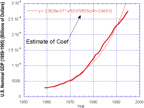
Figure 23: U.S. Nominal GDP (1959-1995)
Goal Seeking Behavior
Chapter 3 discussed the two types of feedback loops that exist in the world: positive loops and negative loops. Positive loops generate exponential growth (or rapid decline) and negative loops produce goal-seeking behavior. This section introduces and analyzes a first order negative feedback loop system.
|
|
Figure 1 presents a generic, first order, linear, negative feedback loop system. The model is initialized in equilibrium by setting the initial value of the stock equal to its goal, and then "shocked" out of equilibrium (at time=1) by a step function that changes the system's goal from ten to fifteen. This procedure -- ie., starting a system dynamics model in equilibrium and then shocking it out -- is widely used in system dynamics because it allows the modeler to see the "pure" behavior of the system in response to the shock. Moreover, it illustrates another important idea in system dynamics modeling: A system containing negative feedback loops will be in equilibrium only when all of its stocks are equal to all of its goals simultaneously.
The implication of this idea is very important. In the real world it is rare, if not impossible, to find actual systems (particularly actual social systems) that exist in states of equilibrium because actual systems contain many negative feedback loops that do not reach their goals simultaneously. Thus, system dynamicists often start their models in states of equilibrium, not because they feel that this reflects reality, but rather because it is a useful reference point for analyzing the "pure" behaviors of their models.
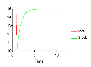
Figure 2: Simulation of the Generic First Order Negative Feedback Loop System in response to a step increase at time=1
The behavior exhibited by the negative feedback loop system as shown in Figure 2 is goal seeking. When the goal is increased from ten to fifteen, a discrepancy between the stock and its goal is created. In response to this discrepancy, the system initiates corrective action by increasing its flow and smoothly raising its stock to a value of fifteen. The time it takes the system to reach its new goal is determined by the size of TimeCoef. The bigger TimeCoef is, the longer it takes for the system to adjust to its new goal. This is illustrated in Figure 3, where the negative feedback loop system of Figure 1 is simulated with three different values of TimeCoef (1, 2, and 3) in response to a reduction in the goal (opposite the case shown in Figures 1 and 2) from ten down to five with a step function at time=1. (Click on image to run simulation)
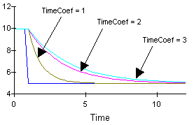
Figure 3: Three Simulations of the Generic First Order Negative Feedback Loop System give a step reduction at time=1
Exact Analytical Solution
To more precisely determine how long it takes a linear first order negative feedback loop system to reach its goal, the exact analytical solution to the model presented in Figure 1 must be studied. This solution is:
To study Equation 1, it is helpful to look at the special case when the system is seeking a goal of zero. Equation 2 presents this special case. It found by simply substituting goal values of zero into Equation 1.
One very important thing to note about Equation 2 is that it is very similar to Equation 1 of Exponential Growth, the exact analytical solution to a linear positive feedback loop system. Indeed, Equations 1 of Exponential Growth and Equation 2 differ only by the signs of their exponents. Equations 1 of Exponential Growth has an exponent of Coef * t and Equation 2 has an exponent of -(1/TimeCoef) * t. Since Coef and 1/TimeCoef are both numbers, the exponents, and hence the equations, differ only by sign. The reason that Equation 2 has a minus sign in front of its exponent is that it represents a system seeking a goal of zero. Thus, under the assumption that the system's stock contains positive values, the system will steadily lose units via its outflow until there is nothing left. This process is known as exponential decay. For the more mathematically inclined reader, the derivation of Equation 1 is presented in the shaded box below.
Derivation of the Analytical Solution to the First Order, Linear, Negative Feedback Loop System. |
|
|
Exponential Decay
Figure 1 below is a system dynamics representation of a linear first order negative feedback loop system with an implicit goal of zero. The figure includes the model's equations, a causal loop diagram, and a simulation of the model's structure. The simulation is an example of exponential decay behavior that corresponds to the exact analytical solution to the system presented in Equation 2 of Goal Seeking Behavior. (Click on image to run simulation)
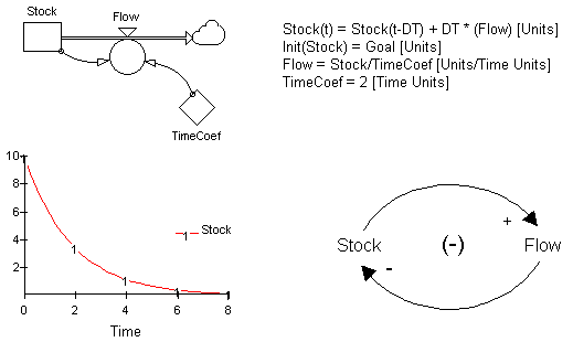
Figure 1: First Order, Linear, Negative Feedback Loop System with an Implicit Goal of Zero
Measures of Exponential Decay: Half Life
One measure of how long it will take for a first order, linear, negative feedback loop system to reach its goal of zero is its half life. The half life of such a system is the time it takes to drain half of the contents from the system's stock. Analogous to the case of the doubling time for a first order positive feedback loop system above, the system's time constant must be determined before its half life can be found.
As was previously shown, the analytical solutions to Equations 1 of Exponential Growth and Equation 2 of Goal Seeking Behavior differ only by sign. It should not be surprising therefore that the equation for the outflow in Figure 1:
Flow = Stock / TimeCoef
�܂���
Flow = Stock * (1/TimeCoef)
is very similar to the equation for the inflow in the Figure 20 of Exponential Growth:
Flow = Stock * Coef
Given that the time constant for the positive feedback loop system of Figure 20 of Exponential Growth is Tc = 1/Coef, and applying the same logic to the negative feedback loop system presented in Figure 1, yields a time constant of Tc = 1/(1/TimeCoef) = TimeCoef. This result can be used to answer a question similar to that asked about the positive feedback loop system: How much progress toward its goal will the negative feedback loop system have made after one time constant has elasped? The answer can be found by substituting the time constant into the Equation 2 of Goal Seeking Behavior:
Stockt = Stock0 * e-(1 / TimeCoef) *Tc
Stockt = Stock0 * e-(1/TimeCoef)*TimeCoef
Stockt = Stock0 * e-1
Stockt = Stock0 * (1/e)
Stockt = Stock0 * .37
This result indicates that the system loses 63% of the contents of its stock after one time constant has elapsed. Extending this logic reveals that the system loses 86% of the contents of its stock after two time constants have elasped (Stockt = Stock0 * .37 * .37 = Stock0 * .14) and 95% of the contents of its stock after three time constants have elapsed (Stockt = Stock0 * .37 * .37 * .37 = Stock0 * .05). Figure 2 repeats the simulation from Figure 1 and confirms this result graphically. As in the case of a first order positive feedback loop system, the negative loop system's half life is 70% of its time constant. That is: Th = .7 * Tc. Once again, the derivation of ths result is presented in the shaded box below for the more methematically inclined reader. A graphical presentation of the result is also shown in Figure 2. (Click on image to run simulation)
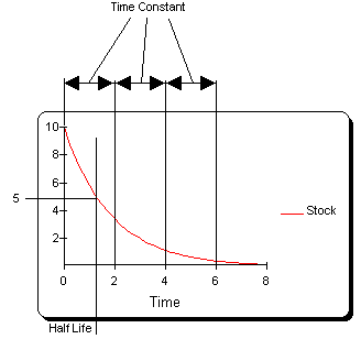
Figure 2: Behavior of a First Order, Linear, Negative Feedback Loop System after Three Time Constants have Elapsed
The analysis of the first order negative feedback loop system with an implicit goal of zero can be extended to the more general negative feedack loop model originally presented in Figure 2 of Goal Seeking Behavior, giving the following insight: A first order, negative, feedback loop system reaches approximately 95% of its goal after three time constants have elapsed.
Derivation of the Half Life for a First Order, Linear, Negative Feedback Loop System |
|
The half life of a first order, linear, negative feeback loop system is calculated using Equation 2 of Goal Seeking Behavior. If the half life, Th, is defined to be the time it takes to cut the initial value of a stock in half, then: 1/2 * Stock0 = Stock0 * e-1/Coef * Th Since the system's time constant, Tc, is 1/Coef, then the system's Coef = 1/Tc. Thus: 1/2 * Stock0 = Stock0 * e-Tc * Th Dividing both sides by Stock0 yields: 1/2 = e - Th/Tc Taking the natural logarithm of both sides yields: ln(1/2) = ln(e -Th/ Tc) �܂��� ln(1) -ln(2) = ln(e-Th/Tc) �܂��� 0 - .69 = - Th / Tc �܂��� .7 = Th / Tc �܂��� Th = .7 * Tc Thus, the half life of a first order, linear, negative feeback loop system is seventy percent of its time constant. |
[Previous] |
[Next] |
 |
Update : 2005/07/23 |