Title : Building Blocks

|
Location : Home > Methods > Simulation > System Dynamics > Introduction to System Dynamics Title : Building Blocks |
|
Seeing System Structure
前セクションでは、時間経路の概念を定義し、これらのシステムの振る舞いのパターンが1つまたは複数の組み合わせからなることを示した。さて、これらの特徴的なパターンの源を検討しよう。特に、集約的システム変数(ストック)と変化率システム変数(フロー)を検討する。システムフィードバックネットワークの基本的な構築ブロックのようにストックとフローが理解しがたく直感的でないような振る舞いをする動的システムを確実にする。さらに、システムの限界を決定する際の非線形関係の役割、フィードバックループの支配力、振る舞いの複雑性に関しても議論する。
Stocks and Flows
システムダイナミクスにおいては、動的な振る舞いは「集積の原則(Principle of Accumulation)」により引き起こされると考えられている。簡単に言えば、この原則は世界の全ての動的な振る舞いはフローがストックに集積されるときに起こると主張している。
図1:簡単なストックとフロー構造の例
たとえを用いれば、図1に示すようにストックはバスタブのようなもので、フローはストックに水を注いだり抜いたりする水道管と蛇口のようなものである。ストック=フロー構造は世界で最も単純な動的システムである。集積の原則に従い、何かが水道管と蛇口を通じてストックに動的な振る舞いは起こる。システムダイナミクスにおいては、情報・非情報の実体がフローを通じて流れ込み、ストックに集積される。
図2は2つのフロー−流入と流出−があるシステムダイナミクスのストック=フロー構造の例である。この例の場合、システムの動的な振る舞いはストックへのフロー、ストックからのフロー(流入−流出)のために起こる。明らかに、流入が流出よりも大きければストックに蓄積されている実体は増加する。流出のほうが大きければストックは減少する。最後に流出と流入が等しければストックの量は同じままである。この最後の可能性はシステムダイナミクスも出るにおける動的平衡の状態を示している。
例2:流入と流出のあるストック=フロー構造の例
原理的には、ストックにはどれだけ流入と流出があってもかまわない。しかしながら現実には、システムダイナミクスモデルには4から6程度以上の流入・流出は見られない。集積の原則は流入・流出の数にかかわらず成立する。
Identifying Stocks and Flows
システムダイナミクスモデルに取り組む者が学ばねばならない基本的なスキルの1つが、自身がモデル化しようとしている問題を表現しているシステムにおいてストックとフローを特定することである。これは容易なことではなく、よく困難に直面する問題でもある。例えば、システムダイナミクスに馴染みのない人たちにとっては、ストックとフローをよく混同する。そのような人は「赤字」(これはフロー)を「負債」(これはストック)だと言う。また、「インフレーション(これはストックへ流入するフロー)は一般価格水準(これはストック)が下落していることである」とも言う。インフレーションの減少とは価格が上昇しているけれどもその上昇率が鈍い状態を指す。
ストックとフローを特定するためには、システムダイナミクスモデルに取り組む者は must determine which 扱う問題を表現しているシステムにおいて、どの変数が状態を定義しているもの(ストック)であり、その変数が状態を変化させているもの(フロー)であるかを決定しなければならない。ストックとフローを特定するには以下に挙げるような指針が有用であろう。
Four Characteristics of Stocks
ストックにはシステムの動的振る舞いを決定するのに重要な4つの特徴がある。簡単に言えばフローは
これらの特徴を順に説明していく。
Stocks have memory
ストックの重要な特徴の1つめは、メモリ(永続性・慣性)を持つことである。これを見るには図1における単純なストック=フロー構造を思い浮かべるとよい。流入を遮断すればストックは増加せず、流入を停止した時点の水準を保持したままである。流入を上回る流出があればストックの量は減少する。この特徴の重要性を過小評価してはならない。ストックへの流入を停止すればストックの量から発生する問題は回避されると人々が信じているが、残念だが、真実は程遠い。
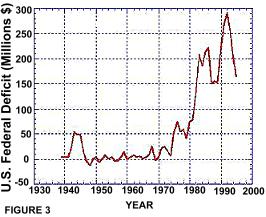
図3:合衆国の財政赤字(1930 - 1993)
合衆国が現在抱えている赤字と負債について考えてみよう。図3は合衆国の赤字額の時系列グラフを示し、図4は負債額の時系列グラフを示している。赤字額は合衆国連邦政府が収入を超過して費やす年間額であるのに対し、, while the 負債は過去のdebt is the accumulation of all the previous deficits (less the debt that has been retired). From an inspection of these figures, it is clear that both the U.S. federal deficit and the U.S. federal debt are growing exponentially.
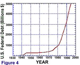
Figure 4: US Federal Debt from 1930 - 1993.
In terms of a simple system dynamics model, the deficit is a flow and the debt is a stock, as shown in Figure 5.*1 Therefore, if the U.S. federal government were to balance its budget (i.e., make the deficit inflow zero), the debt would not decrease at all. This fact is surprising to many people!
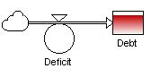
Figure 5: Structure of US Debt/Deficit problem.
A similar case involves the depletion of the earth's ozone layer. In 1990 the nations of the world agreed to a ban on the production (and hence on the eventual release into the atmosphere) of ozone-killing chlorofluorocarbons (CFC's).
Figure 6: System dynamics structure of CFC accumulation in atmosphere.
From a system dynamics point of view, this agreement caused the flow of chlorofluorocarbons into the atmosphere to stop, but did nothing to remove any of the chlorofluorocarbons already in the atmosphere and destroying ozone (a stock -- see Figure 6). The removal of these pollutants can only be accomplished via the earth's natural cleansing processes. *2
Stocks Change the Time Shape of Flows
A second important characteristic of stocks is that they (i.e., the accumulation process) usually change the time shape of flows.*3 This can be seen by simulating the simple stock-flow structure shown in Figure 1, with different time shapes for the flow. Figure 7 for example, presents the time shape of the stock when the flow is at a constant level of 5 units/time. An examination of the figure reveals that the accumulation process changes the horizontal time shape of the flow into a linear growth shape for the stock. *4
(Click on image to see animation)
In a similar way, Figure 8 through Figure 13 show the time shape of the stock for different time shapes exhibited by the flow.
(Click on image to see animation)
In Figure 8, we see that if the inflow valve is "opened" or increases in a linear fashion, (i.e., a linear growth shape that is at all times positive), the "level" of the stock variable will grow at an increasing rate.
(Click on image to see animation)
Figure 9 shows that a linear decline shape for the inflow, which is at all times positive, causes the stock to grow at a decreasing rate. Recall the example above in which a decrease in inflation reduced the rate of increase in price. In this case, price would be analogous to the stock variable and rate of inflation would be the analogous to the inflow variable.
(Click on image to see animation)
In figure 10, we see a case in which the inflow (valve) is at all time negative. This is equivalent to saying that the inflow valve is "drawing down the level" (i.e., it's a drain). In this case, the time path for the inflow valve is at all times negative and is declining linearly. This causes the stock to decline at an increasing rate.. *5
(Click on image to see animation)
The case shown in Figure 11 is similar to that of Figure 10 in that the inflow valve is always negative, indicating that the stock is being drawn down. However, in this case the flow valve is closing, i.e., becoming less negative. As show in the figure, a linear growth shape for the flow, which is at all times negative, causes the stock to decrease at a decreasing rate.
(Click on image to see animation)
Figure 12 illustrates case in which "shape" of the inflow time path is not changed by the accumulation process.*6 In this case, an inflow that increases exponentially causes the stock (the accumulation ) to increase in a similar fashion.*7 In terms of real-world stock and flow data, the National deficit and debt data shown in Figure 3 and Figure 4 illustrate this case.
(Click on image to see animation)
In Figure 13, we see the result of having the inflow oscillating in a sinusoidal manner between a value of 1 and -1, i.e., the stock is being filled and drained repeatedly. As one would expect, the stock mimics the inflow's time path character (as in Figure 12). It is important to note, however, that maximum value of the stock is reached after the inflow's maximum.*8
Stocks decouple flows
A third important characteristic of stocks is that they "decouple" or interrupt flows. A stock thus makes it possible for an inflow to be different from an outflow and hence for disequilibrium behavior to occur.*9 In addition, the decoupling of flows by stocks makes it possible for inflows to be controlled by sources of information that differ from those controlling outflows. Figure 14 shows a number of examples in which flows are decoupled by stocks.
Figure 14: Examples where flows are decoupled by stocks
Stocks create delays
A fourth important characteristic of stocks is that they create delays. This can be seen by re-examining Figure 13 -- the response of a stock to a sinusoidal inflow. In this example, it is clear that the stock reaches each of its peaks and troughs after the flow reaches each of its corresponding peaks and troughs, during each repetition of the cycle. Henri Bergson once remarked that "time is a device that prevents everything from happening at once".*10 Bergson's point of course is that, despite human impatience, events in the world do not occur instantaneously. Instead, there is often a significant lag between cause and effect. In system dynamics modeling, identifying delays is an important step in the modeling process because they often alter a system's behavior in significant ways. The longer the delay between cause and effect, the more likely it is that a decision maker will not perceive a connection between the two. Figure 15 presents some examples of stock-flow structures specifying significant system delays.
Figure 15: Examples of Stock-Flow Structures Specifying Significant System Delays
Feedback
A lthough stocks and flows are both necessary and sufficient for generating dynamic behavior, they are not the only building blocks of dynamical systems. More precisely, the stocks and flows in real world systems are part of feedback loops, and the feedback loops are often joined together by nonlinear couplings that often cause counterintuitive behavior.
From a system dynamics point of view, a system can be classified as either "open" or "closed." Open systems have outputs that respond to, but have no influence upon, their inputs. Closed systems, on the other hand, have outputs that both respond to, and influence, their inputs. Closed systems are thus aware of their own performance and influenced by their past behavior, while open systems are not.
Of the two types of systems that exist in the world, the most prevalent and important, by far, are closed systems. As shown in Figure 1, the feedback path for a closed system includes, in sequence, a stock, information about the stock, and a decision rule that controls the change in the flow. Figure 1 is a direct extension of the simple stock and flow configuration shown previously with the exception that an information link added to close the feedback loop. In this case, an information link "transmits" information back to the flow variable about the state (or "level") of the stock variable. This information is used to make decisions on how to alter the flow setting.
Figure 1: Simple System Dynamics Stock-Flow-Feedback Loop Structure.
It is important to note that the information about a system's state that is sent out by a stock is often delayed and/or distorted before it reaches the flow (which closes the loop and affects the stock). Figure 2, for example, shows a more sophisticated stock-flow-feedback loop structure in which information about the stock is delayed in a second stock, representing the decision maker's perception of the stock (i.e., Perceived_Stock_Level), before being passed on. The decision maker's perception is then modified by a bias to form his or her opinion of the stock (i.e., Opinion_Of_Stock_Level). Finally, the decision maker's opinion is compared to his or her desired level of the stock, which, in turn, influences the flow and alters the stock.
Given the fundamental role of feedback in the control of closed systems then, an important rule in system dynamics modeling can be stated: Every feedback loop in a system dynamics model must contain at least one stock.
Figure 2: More Sophisticated Stock-Flow-Feedback Loop Structure
Positive and Negative Loops
Closed systems are controlled by two types of feedback loops: positive loops and negative loops. Positive loops portray self-reinforcing processes wherein an action creates a result that generates more of the action, and hence more of the result. Anything that can be described as a vicious or virtuous circle can be classified as a positive feedback process. Generally speaking, positive feedback processes destabilize systems and cause them to "run away" from their current position. Thus, they are responsible for the growth or decline of systems, although they can occasionally work to stabilize them.
Negative feedback loops, on the other hand, describe goal-seeking processes that generate actions aimed at moving a system toward, or keeping a system at, a desired state. Generally speaking, negative feedback processes stabilize systems, although they can occasionally destabilize them by causing them to oscillate.
Causal Loop Diagramming
In the field of system dynamics modeling, positive and negative feedback processes are often described via a simple technique known as causal loop diagramming. Causal loop diagrams are maps of cause and effect relationships between individual system variables that, when linked, form closed loops.
|
Figure 3, for example, presents a generic causal loop diagram. In the figure, the arrows that link each variable indicate places where a cause and effect relationship exists, while the plus or minus sign at the head of each arrow indicates the direction of causality between the variables when all the other variables (conceptually) remain constant. More specifically, the variable at the tail of each arrow in Figure 3 causes a change in the variable at the head of each arrow, ceteris paribus, in the same direction (in the case of a plus sign), or in the opposite direction (in the case of a minus sign). |
|
The overall polarity of a feedback loop -- that is, whether the loop itself is positive or negative -- in a causal loop diagram, is indicated by a symbol in its center. A large plus sign indicates a positive loop; a large minus sign indicates a negative loop. In Figure 3 the loop is positive and defines a self reinforcing process. This can be seen by tracing through the effect of an imaginary external shock as it propagates around the loop. For example, if a shock were to suddenly raise Variable A in Figure 3, Variable B would fall (i.e., move in the opposite direction as Variable A), Variable C would fall (i.e., move in the same direction as Variable B), Variable D would rise (i.e., move in the opposite direction as Variable C), and Variable A would rise even further (i.e., move in the same direction as Variable D).
|
By contrast, Figure 4 presents a generic causal loop diagram of a negative feedback loop structure. If an external shock were to make Variable A fall, Variable B would rise (i.e., move in the opposite direction as Variable A), Variable C would fall (i.e., move in the opposite direction as Variable B), Variable D would rise (i.e., move in the opposite directionas Variable C), and Variable A would rise (i.e., move in the same direction as Variable D). The rise in Variable A after the shock propagates around the loop, acts to stabilize the system -- i.e., move it back towards its state prior to the shock. The shock is thus counteracted by the system's response. |
|
|
Occasionally, causal loop diagrams are drawn in a manner slightly different from those shown in Figure 3 and Figure 4. More specifically, some system dynamicists prefer to place the letter "S" (for Same direction) instead of a plus sign at the head of an arrow that defines a positive relationship between two variables. The letter "O" (for Opposite direction) is used instead of a minus sign at the head of an arrow to define a negative relationship between two variables. To define the overall polarity of a loop system dynamicists often use the letter "R" (for "Reinforcing") or an icon of a snowball rolling down a hill to indicate a positive loop. To indicate a negative loop, the letter "B" (for "Balancing"), the letter "C" (for "Counteracting"), or an icon of a teetertotter is used. Figure 5 illustrates these different causal loop diagramming conventions. |
|
In order to make the notion of feedback a little more salient, Figure 6 to Figure 17 present a collection of positive and negative loops. As these loops are shown in isolation (i.e., disconnected from the other parts of the systems to which they belong), their individual behaviors are not necessarily the same as the overall behaviors of the systems from which they are taken.
Positive Feedback Examples
| Population Growth/Decline: Figure 6 shows the feedback mechanism responsible for the growth of an elephant herd via births. In this simple example we consider two system variables: Elephant Births and Elephant Population. For a given elephant herd, we say that if the birth rate of the herd were to increase, the Elephant Population would increase. In this same way, we can say that if - over time - the Elephant Population of the herd were to increase, the birth rate of the herd would increase. Thus, the Elephant Birth rate drives the Elephant Population that drives Elephant Birth rate - positive feedback. |
|
|
National Debt: Figure 7 is a positive loop that shows the growth in the national debt due to the compounding of interest payments. First, we note that that an increase in the amount of interest paid per year on the national debt (itself a cost within the federal budget ) will cause the overall national debt to increase. In this same way, an increase in the level of national debt will increase the amount of the interest paid each year. |
|
| Arms Race: Figure 8 shows a generic arms race between Country A and Country B. In its simplest form, an "arms race" can be described as a self-sustaining competition for military superiority. An arms race is driven by the perception that one's adversary has equal or greater military strength. If Country A moves to increase its military capability, Country B interprets this as a threat and responds in-kind with its own increase in military capability. Country B's action, in turn, causes Country A to feel more threatened. Thus, Country A moves to further increase its military capability. |
|
|
Bank Panic: A common scene during the Great Depression in the 1930s was that of a panic stricken crowd standing outside their local bank waiting to withdraw what remained of their savings. Figure 8 shows the feedback mechanism responsible for the spiraling decline of the banking system during this period. From the diagram, we see that the frequency of bank failures increases public concern and the fear of losing their money. In this case, we say that the two system variables "move" in the same (S) or positive (+) direction. The relationship between the "fear of not being able to withdraw money" and the rate at which bank withdrawals are made is also positive. |
|
The relationship between withdrawals and bank health is negative (-) or opposite (O). This means that if the rate of bank withdrawals increases, the health of the bank decreases as capital reserves are drawn down. The relationship between the banking industry's health and the rate of bank failures is also negative. This means that if the health of the banking industry increases, the number of bank failures per year will decrease.
This vicious cycle was clearly seen during the 1930s. An overall economic downturn caused the rate of bank failures to increase. As more banks failed, the public's fear of not being able to withdraw their own money increased. This, in turn, prompted many to withdraw their savings from banks, which further reduced the banking industry's capital reserves. This caused even more banks to fail.
|
Figure 10 depicts three interacting positive feedback loops that are thought to be responsible for the growth in students taking drugs in high school. |
|
Negative Feedback Examples
|
Population Growth/Decline:In Figure 6, we saw how an elephant population and its corresponding birth rate form a positive feedback loop. Now, we consider the other half of the equation, that is, the feedback structure between Elephant Population and Elephant Death rate. Figure 11 shows the negative feedback process responsible for the decline of an elephant herd via deaths. If the Elephant Death rate increases, the Elephant Population will decrease. A negative sign indicates this counteracting behavior. The causal influence of Elephant Population to Elephant Death rate is just the opposite. An increase in the number of elephants in the herd means that a proportionally larger number of elephants will die each year, i.e., an increase in the herd's death rate. A plus sign indicates this complimentary behavior. These two relationships combine together to form a negative feedback loop. |
|
|
Figure 12 and Figure 13 are two simple and familiar examples of negative feedback processes. Figure 12 shows the negative feedback process responsible for the dissipation of Itching due to Scratching. Figure 13 considers the negative feedback involved in Eating to reduce Hunger. An increase in one's Hunger causes a person to eat more food. Increasing in the rate food consumption, in turn, reduces Hunger. | |
|
|
|
| Law Enforcement:Figure 14 depicts a negative feedback process that maintains a balance between the number of drug dealers and the number of police officers in a neighborhood. An increase in the number of drug dealers in a neighborhood will prompt local officials to increase the number of law enforcement persons as a counter measure. As the number of police officers increase, more arrests are made and the number of drug dealers is reduced. |
|
Car Pools:Figure 15 shows a negative feedback process that maintains a balance between car pools and gasoline consumption. An increase in gasoline consumption increases gasoline price (supply reduction). A higher gasoline price pushes many individual motorists to join carpools, which reduces the total number of vehicles on the road. This, in turn, reduces gasoline consumption. |
|
Implicit and Explicit Goals
The negative feedback loops presented in Figure 11 through Figure 15 are, in a sense, misleading because the goals they are seeking are implicit rather than explicit. For example, the implicit goal of the loop in Figure 11 is zero elephants. That is, if the loop were to act, in isolation, for a substantial period of time, eventually all of the elephants would die and the population would be zero. The same sort of logic applies to Figure 12 and Figure 13, in which the loops implicitly seek goals of zero itching and zero hunger respectively.The logic gets even murkier in the case of Figure 14 and Figure 15. In Figure 14, there is an implicit goal of an "acceptable" or "tolerable" level of drug dealers in the neighborhood, which may or may not be zero. In Figure 15, there is an implicit goal of an acceptable or tolerable gasoline price, which is certainly a lower price rather than a higher price, but is also (realistically) not zero.
Figure 16: Generic negative feedback structure with explicit goal
An alternative and (often) more desirable way to represent negative feedback processes via causal loop diagrams is by explicitly identifying the goal of each loop. Figure 16, for example, shows a causal loop diagram of a generic negative feedback structure with an explicit goal. The logic of this loop says that, any time a discrepancy develops between the state of the system and the desired state of the system (i.e., goal), corrective action is called forth that moves the system back into line with its desired state.
A more concrete example of a negative feedback structure with an explicit goal is shown in Figure 17. In the figure, a distinction is drawn between the actual number of elephants in a herd and the desired number of elephants in the herd (presumably determined by a knowledge of the carrying capacity of the environment supporting the elephants). If the actual number of elephants begins to exceed the desired number, corrective action -- i.e., hunting -- is called forth. This action reduces the size of the herd and brings it into line with the desired number of elephants.
Figure 17: Example of negative feedback structure with an explicit goal
Examples of Interacting "Nests" of Positive and Negative Loops
In system dynamics modeling, causal loop diagrams are often used to display "nests" of interacting positive and negative feedback loops. This is usually done when a system dynamicist is attempting to present the basic ideas embodied in a model in a manner that is easily understood, without having to discuss in detail.
As Figure 18 and Figure 19 show, when causal loop diagrams are used in this fashion, things can get rather complicated. Figure 18 is a causal loop diagram of a system dynamics model created to examine issues related to profitability in the paper and pulp industry. This figure has a number of features that are important to mention. The first is that the authors have numbered each of the positive and negative loops so that they can be easily referred to in a verbal or written discussion. The second is that the authors have taken great care to choose variable names that have a clear sense of direction and have real-life counterparts in the actual system. The last and most important feature is that, although the figure provides a sweeping overview of the feedback structure that underlies profitability problems in the paper and pulp industry, it cannot be used to determine the dynamic behavior of the model (or of the actual system). In other words, it is impossible for someone to accurately think through, or mentally simulate, the dynamics of the paper and pulp system from Figure 18 alone.
Figure 18: Causal Loop Diagram of a Model Examining Profitability in the Paper and Pulp Industry
Figure 19 is a causal loop diagram of a system dynamics model created to examine forces that may be responsible for the growth or decline of life insurance companies in the United Kingdom. As with Figure 18, a number of this figure's features are worth mentioning. The first is that the model's negative feedback loops are identified by "C's," which stand for "Counteracting" loops. The second is that double slashes are used to indicate places where there is a significant delay between causes (i.e., variables at the tails of arrows) and effects (i.e., variables at the heads of arrows). This is a common causal loop diagramming convention in system dynamics. Third, is that thicker lines are used to identify the feedback loops and links that author wishes the audience to focus on. This is also a common system dynamics diagramming convention. Last, as with Figure 18, it is clear that a decision maker would find it impossible to think through the dynamic behavior inherent in the model, from inspection of Figure 19 alone.
Figure 19: Causal Loop Diagram of a Model Examining the Growth or Decline of a Life Insurance Company.
Archetypes
An area of the field of system dynamics or, more precisely, of the much broader field of "systems thinking," that has recently received a great deal of attention is archetypes. Archetypes are generic feedback loop structures, presented via causal loop diagrams, that seem to describe many situations that frequently appear in public and private sector organizations. Archetypes are thought to be useful when a decision maker notices that one of them is at work in his or her organization. Presumably, the decision maker can then attack the root causes of the problem from an holistic and systemic perspective. Currently, nine archetypes have been identified and cataloged by systems thinkers, including:
Recent efforts, however, have suggested that the number can be reduced to four:
No matter what the true number archetypes is or will be, however, the central question remains unanswered: How successful are archetypes in helping decision makers solve problems in their organizations?
Problems with Causal Loop Diagrams
Causal loop diagrams are an important tool in the field of system dynamics modeling. Almost all system dynamicists use them and many system dynamics software packages support their creation and display.
Although some system dynamicists use causal loop diagrams for "brainstorming" and model creation, they are particularly helpful when used to present important ideas from a model that has already been created. The only potential problem with causal loop diagrams and archetypes then, occurs when a decision maker tries to use them, in lieu of simulation, to determine the dynamics of a system.
Causal loop diagrams are inherently weak because they do not distinguish between information flows and conserved (noninformation) flows. As a result, they can blur direct causal relationships between flows and stocks. Further, it is impossible, in principle, to determine the behavior of a system solely from the polarity of its feedback loops, because stocks and flows create dynamic behavior, not feedback. Finally, since causal loop diagrams do not reveal a system's parameters, net rates, "hidden loops," or nonlinear relationships, their usefulness as a tool for predicting and understanding dynamic behavior is further weakened. The conclusion is that simulation is essential if a decision maker is to gain a complete understanding of the dynamics of a system.
Nonlinearity
A large part of the system dynamics modeling process involves the application of common sense to dynamic problems. A good system dynamic modeler is always on the look-out for model behaviors that do not make sense. Such behaviors usually indicate a flaw in a model, and the flaw is often that a crucial piece of system structure has been left out of the model. A common error that novice system dynamicists make is to build models with stocks whose values can either go negative, or run off to infinity. Common sense, of course, dictates that no real system can grow infinitely large, and hence that no model of a real system should be able to grow infinitely large. Similarly, common sense suggests that, since many real world variables cannot take on negative values, their model-based counterparts should not be able to take on negative values. When a system dynamicist looks for relationships in an actual system that prevent its stocks from going negative or growing infinitely large, he or she is usually looking for the system's nonlinearities. Nonlinear relationships usually define a system's limits. Nonlinear relationships play another important role in both actual systems and system dynamics modeling. Frequently, a system's feedback loops will be joined together in nonlinear relationships. These nonlinear "couplings" can cause the dominance of a system's feedback loops to change endogenously. That is, over time, a system whose behavior is being determined by a particular feedback loop, or set of loops, can (sometimes suddenly) endogenously switch to a behavior determined by another loop or set of loops. This particular characteristic of nonlinear feedback systems is partially responsible for their complex, and hard-to-understand, behavior. As a result, system dynamics modeling involves the identification, mapping-out, and simulation of a system's stocks, flows, feedback loops, and nonlinearities.
【原注】
[Previous] |
[Next] |
|
|
Updated : 2006/02/07 |
 Figure 4: Generic causal loop diagram of a negative feedback loop structure

 Figure 9: Bank panic is a positive feedback process.