Title : Chapter 6 : Natural Gas Discovery

|
Location : Home > Methods > Simulation > System Dynamics > Introduction to System Dynamics Title : Chapter 6 : Natural Gas Discovery |
 |
Natural Gas Discovery
As we discussed in the System Dynamics and Energy Modeling section, one of the system dynamics analyses conducted in support of the world modeling efforts was a natural gas discovery and production model created by MIT Master's student Roger Naill. Naill based his model on the life cycle theory of oil and gas discovery and production put forth by petroleum geologist M. King Hubbert. Like Hubbert, Naill assumed for his analysis that the total amount of oil and gas in the United States (i.e., the amount of oil and gas "in place"), and hence the "ultimately recoverable" amount of oil and gas in the United States, is finite. In this chapter, we recreate Naill's original Natural Gas Discovery Model as a case study in how to construct and experiment with system dynamics models. To make the explanation of the model more manageable, we present a series of model versions, each version incrementally more complex with the addition of new structure. In each case, the reader is encouraged to run the model to see how the additional structure affects its behavior. In the final section of this chapter, we present a "flight simulator" version of the completed model. The reader is encouraged to conduct policy experiments by changing decision variables or model uncertainty variables to see how the behavior of the system changes in response.
Natural Gas Discovery Model: Reference Modes
It is often argued that system dynamics modeling is mis-named because system dynamicists model problems, not systems. The reason that problems, rather than systems, are focused on is because they direct the system dynamicist away from the "kitchen sink approach" to modeling, which usually yields a model containing so much detail that it is no more easy to understand than the actual system itself. The principle way that system dynamicists force themselves to focus on problems is through the use of reference modes. Reference modes are time series graphs of important system variables that exhibit patterns of behavior (e.g., exponential growth, exponential decay, oscillation, s-shaped growth, overshoot and collapse ) that are either problematic or not well understood. They also define the time horizon of a model, which involves the specification of both its time units (years, quarters, months, weeks, days, etc.) and time span (the model’s start time and stop time). The task of the system dynamicist is to identify, and include in the model, only those variables that help to explain (i.e., help the model to mimic) the reference modes. The reference modes originally used by Roger Naill in the construction of his natural gas model were drawn from the oil and gas life cycle theory of M. King Hubbert. Hubbert based his theory on the knowledge of the physical structure of the oil and gas system and hence on the assumption that there is a finite amount of oil and gas in the earth. According to Hubbert’s theory, the discovery and production flows of natural gas, as well as the stock of proven reserves of natural gas rise, peak and fall over time, and the stock of unproven resources falls monotonically due to depletion. Although a theory can be used to provide reference modes for a system dynamics model, actual numerical time series data, if available, can also be used. Figure 1 presents some actual data from the U.S. natural gas system. It includes the actual discovery rate, usage (production) rate, proven reserves, and reserve-production ratio. Clearly, these data do not span the entire life cycle of the natural gas system (roughly the years 1900 to 2050) a la Hubbert, so they are of limited use in specifying reference modes for the natural gas depletion problem. On the other hand, they can be used to complement the reference modes resulting from Hubbert’s theory and to calibrate the model.
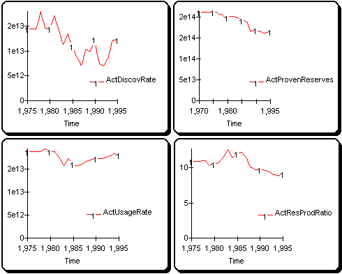
Figure 1: Actual Data from the U.S. Natural Gas Discovery and Production System
Step-By-Step Re-Creation of the Natural Gas Discovery and Production Model
A good way to gain an understanding of a system dynamics model created by another person, is through a step-by-step replication of its structure. In this section, Roger Naill's model of U.S. natural gas discovery and production will be recreated through a series of increasingly sophisticated system dynamics models. To augment the discussion, you can access and run each model version directly. Simulating the models will allow you to see the effect of adding complexity to the base model structure.
First Cut
Figure 1 is the stock-flow diagram for the first step in the recreation of Naill’s model of U.S. natural gas discovery and production. The model consists of two stocks: UnprovenReserves and ProvenReserves, and two flows: DiscoveryRate and UsageRate. The UsageRate is roughly equivalent to the rate of production of U.S. natural gas. One feature of the model that is particularly noteworthy is that there is no inflow to the stock of UnprovenReserves. This is because natural gas is created in geologic time, yet used on a human time scale of a hundred years or so. Thus, for all practical purposes, the amount of natural gas in the United States can be treated as fixed. Naill made this assumption because he based his model on the resource life cycle theory of M. King Hubbert. A fixed stock of gas or oil is at the core of Hubbert’s theory.

Figure 1: First Cut of Naill’s Model of U.S. Natural Gas Discovery and Production
Figure 2 lists the system dynamics equations that directly correspond to the icons shown in Figure 1. Three features of these equations are important to note. The first is that the variables on the left hand side of each equal sign have their measurement units enclosed in brackets {}. In system dynamics modeling stocks are measured in "units" and flows are measured in "units/time." In Figure 2, each of the stocks is measured in "Cubic Feet" of gas and each of the flows is measured in "Cubic Feet (of gas)/Year." In system dynamics modeling, each of the equations in a model must be "dimensionally correct." This means that the arithmetic of the units of measurement must be correct. For example, if a flow {units/time} is equal to a stock {units} divided by a constant, the constant must be measured in {time}. Inspection of the equations in Figure 2 reveals that they are all dimensionally correct. The second feature of the equations in Figure 2 is that the stocks each have initial values. More specifically, the initial amount of gas in the stock of UnprovenReserves is 6.4*e12 cubic feet and the initial amount of gas in the stock of ProvenReserves is 1.28434*e15 cubic feet. The initial values of stocks in system dynamics models can be determined in a variety of ways. The values are often known or knowable and the analyst needs only to investigate available data sources to find out. In the case of Naill’s model presented here, the initial values were estimated by using the system dynamics software to calculate the "best fit" to actual U.S. natural gas discovery and production data. In the case of UnprovenReserves, a value estimated by Hubbert’s method could also have been used. The third feature of the equations in Figure 2 is that both of the flows have first order control. This means that a negative or balancing feedback loop has been created between each stock and its outflow to prevent the stocks from ever taking on negative values (because "negative UnprovenReserves" and "negative ProvenReserves" would not make sense). An examination of the equations reveals that, when either UnprovenReserves or ProvenReserves reach a value of zero, their outflows are shut off (i.e., take on values of zero).
|
[Stock] ProvenReserves = dt*(DiscoveryRate - UsageRate {Cubic Feet} [Initial] ProvenReserves = 6.4e12 {Cubic Feet} [Stock] UnprovenReserves = dt*(-DiscoveryRate) {Cubic Feet} [Initial] UnprovenReserves = 1.28434e15 {Cubic Feet} [Flow] DiscoveryRate = UnprovenReserves*DiscoveryCoef {Cubic Feet/Year} [Flow] UsageRate = ProvenReserves*UsageCoef {Cubic Feet/Year} [Constant] DiscoveryCoef = .0075 {1/Years} [Constant] UsageCoef = .02 {1/Years} |
Figure 3 shows time series plots from a simulation of the model presented in Figures 1 and 2. Of note is that, even at this very early stage in the model’s development, it produces dynamic behavior consistent with the real system. UnprovenReserves fall monotonically due to depletion and ProvenReserves rise during the early part of the century, peak during the mid-1970s, and then decline thereafter. The DiscoveryRate falls monotonically and the UsageRate (essentially the production rate) rises from 1900 to the mid-1970s, peaks, and then declines thereafter.
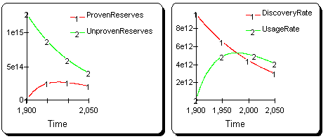
Figure 3: Time Series Plots from a Simulation of Naill’s Model of U.S. Natural Gas Discovery and Production
Second Cut
Figures 4(a) and 4(b) illustrate the stock-flow and causal diagrams for the second step in the recreation of Naill’s model of U.S. natural gas discovery and production. The model is merely an extension of the model presented in Figure 1.
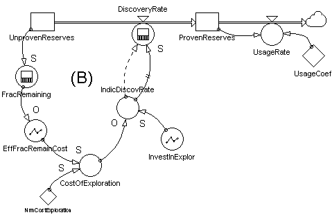
Figure 4(a): Second Cut of Naill’s Model of U.S. Natural Gas Discovery and Production
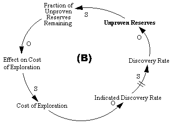
Figure 4(b): Causal Diagram the the Second Cut of Naill's Model
of U.S. Natural Gas Discovery and Production.
A comparison of Figure 4(a) to Figure 1 reveals that the right-hand side of the model (ProvenReserves, UsageRate, UsageCoef) has not changed. The left-hand side of the model, on the other hand, has had a significant piece of system dynamics structure added to it. More precisely, the simple discovery rate equation has been replaced by a balancing feedback loop (negative feedback) that works its way through the fraction of unproven reserves remaining and the cost of exploration. Refering to Figure 4(b), the logic of the balancing loop is as follows: a fall in unproven reserves (UnprovenReserves), ceteris paribus, causes a fall (i.e., a move in the Same direction) in the fraction of unproven reserves remaining (FracRemaining). A fall in the FracRemaining, ceteris paribus, causes a rise (i.e., a move in the Opposite direction) in the effect of the fraction remaining on the cost of exploration (EffFracRemainCost). A rise in the EffFracRemainCost, ceteris paribus, causes a rise in the cost of exploration (CostOfExploration). A rise in the CostOfExploration, ceteris paribus, causes a fall in the indicated discovery rate (IndicDiscovRate) which, in turn, ceteris paribus, causes a fall in the discovery rate (DiscoveryRate). A fall in the DiscoveryRate closes the loop and ensures, ceteris paribus, that unproven reserves will be higher than they otherwise would have been. Three other features of the model presented in Figure 4a are important to note. The first is that the balancing loop preserves first order control in the model. That is, although the feedback from the stock of unproven reserves to its outflow (DiscoveryRate) is not direct as it was in the first cut of the model, the equations in the loop still causes the computer to shut-off the discovery rate when the stock of unproven reserves is zero. The second feature of the model presented in Figure 4a that is important to note is the delay symbol that appears in the discovery rate icon. The purpose of embedding a delay in the discovery rate is to account for the lag that exists between the time a decision is made to invest in gas exploration and the time actual gas discoveries occur. This delay could also have been modeled explicitly with a simple stock and flow stucture. The last feature of the model that is important to note is its table functions. Represented by the zig-zag-like symbols, table functions allow the modeler to externally impose relationships(linear and nonlinear) between system variables. Figure 5 lists the system dynamics equations that directly correspond to the icons shown in Figure 4. Three characteristics of these equations are particularly noteworthy. The first is that, in addition to the stocks(rectangles), flows (pipe and faucet assemblies) and constants (diamonds) presented in the first cut of the model, there are now auxiliary equations (circles) in the model. The second noteworthy characteristic is that the model is again dimensionally correct. In particular, the measurement units of each variable in the balancing loop correspond to the arithmetic embodied in each equation in the loop. To provide just one example, the indicated discovery rate (Cubic Feet/Year) is equal to investment in exploration (Dollars/Year) divided by the cost of exploration (Dollars/Cubic Foot). The third noteworthy characteristic is that two of the auxiliaries contain table functions (EffFracRemainCost and InvestInExplor) in nongraphical form. The graphical versions of these functions are shown in Figure 6.
|
[Stock] ProvenReserves = dt*(DiscoveryRate - UsageRate) {Cubic Feet} [Initial] ProvenReserves = 6.4e12 {Cubic Feet} [Stock] UnprovenReserves = dt*(-DiscoveryRate) {Cubic Feet} [Initial] UnprovenReserves = 1.28434e15 {Cubic Feet} [Flow] DiscoveryRate = DELAYINF(IndicDiscovRate,4.5,3) {Cubic Feet/Year} [Flow] UsageRate = ProvenReserves*UsageCoef {Cubic Feet/Year} [Aux] CostOfExploration = NrmCostExploration*EffFracRemainCost {Dollars/Cubic Foot} [Aux] EffFracRemainCost = GRAPH(LN(10*FracRemaining),-3.5,0.5,[13000,6000,2700,1000,545,245,110,50, 22,9.98,4.48,2.02,0.91"Min:0;Max:13000;Zoom"]) {Dimensionless} [Aux] FracRemaining = UnprovenReserves/INIT(UnprovenReserves) {Dimensionless} [Aux] IndicDiscovRate = InvestInExplor/CostOfExploration {Cubic Feet/Year} [Aux] InvestInExplor = GRAPH(TIME,1900,15,[100000000,220000000,350000000,470000000, 600000000,720000000,820000000,900000000,950000000,990000000, 1000000000"Min:0;Max:1000000000;Zoom"]) {Dollars/Year} [Constant] NrmCostExploration = 1.34775e-5 {Dollars/Cubic Foot} [Constant] UsageCoef = .02 {1/Years} |
An examination of Figure 6 reveals that the table functions both represent nonlinear relationships in the model and help to define the system’s limits. The effect of the fraction of gas remaining on the exploration cost function (EffFracRemainCost) indicates that as gas depletion occurs, the cost of gas exploration increases monotonically. The investment in exploration function (InvestInExplor) indicates that, over time, the number of dollars per year allocated to gas exploration increases and then saturates. In future cuts of the model, this relationship will be made endogenous.
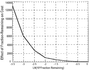
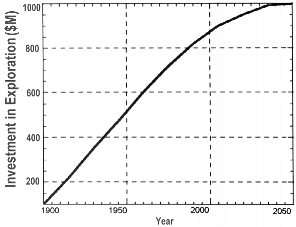
Figure 6: Table Functions in the Second Cut of Naill’s Model of U.S. Natural Gas Discovery and Production
Figure 7 shows time series plots from a simulation of the model presented in Figures 4 and 5. As with the previous version of the model, this cut produces dynamic behavior consistent with the real system. That is, the UsageRate again rises from 1900 to the mid-1970s, peaks, and then declines. UnprovenReserves again fall monotonically due to depletion and ProvenReserves again rise during the early part of the century, peak during the mid-1970s, and then decline. The only behavior in this version of the model that is new involves the DiscoveryRate. A comparison of Figures 3 and 7 reveals that the DiscoveryRate now rises and falls whereas, in the previous version of the model, it simply fell monotonically. The reason for this difference is that, in this cut of the model, the InvestInExplor table function exogenously increases investment in exploration over time. Early in the system’s evolution, the increasing amount of investment dollars causes a rise in natural gas discovery. Later on, however, the effects of depletion overwhelm the investment dollars and the discovery rate falls. An interesting simulation experiment that could be done is to systematically alter the InvestInExplor function (its shape, its saturation level, etc.) and resimulate the model to ascertain the results of the changes.
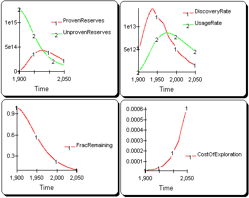
Figure 7: Time Series Plots from a Simulation of the Second Cut of Naill’s Model of U.S. Natural Gas Discovery and Production
Third Cut
Figure 8(a)and 8(b) correspond to the stock-flow and causal diagram for the third step in the re-creation of Naill’s model of U.S. natural gas discovery and production. The model is a direct extension of the model presented in Figures 4 and 5. Four significant changes were made to the second cut of Naill's model in order to arrive at this version of the natural gas system:
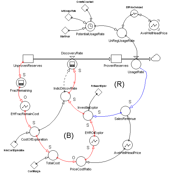
Figure 8(a): Third Cut of Naill’s Model of U.S. Natural Gas Discovery and Production
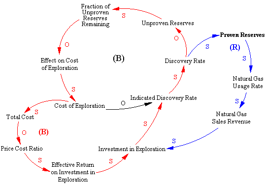
Figure 8(b): Causal Diagram of additional balancing and reinforcing loops.
The logic of the balancing loop, shown in red, is as follows. A fall in UnprovenReserves, ceteris paribus, causes a fall in FracRemaining. A fall in the FracRemaining, ceteris paribus, causes a rise in the EffFracRemainCost. A rise in the EffFracRemainCost, ceteris paribus, causes a rise in the CostOfExploration. A rise in the CostOfExploration, ceteris paribus, causes a rise in the total cost of natural gas (TotalCost). A rise in the TotalCost, ceteris paribus, causes a fall in the ratio of gas price to gas cost (PriceCostRatio). A fall in the PriceCostRatio, ceteris paribus, causes a fall in the effect of return on investment in exploration (EffROIExplor). A fall in EffROIExplor, ceteris paribus, causes a fall in InvestInExplor. A fall in InvestInExplor, ceteris paribus, causes a fall in the IndicDiscovRate which, in turn, ceteris paribus, causes a fall in the DiscoveryRate. A fall in the DiscoveryRate closes the loop and ensures, ceteris paribus, that unproven reserves will be higher than they otherwise would have been. The logic of the reinforcing loop,shown in blue, is as follows. A rise in proven reserves (ProvenReserves), ceteris paribus, causes a rise in the natural gas usage rate (UsageRate). A rise in the UsageRate, ceteris paribus, causes a rise in revenue from the sales of natural gas (SalesRevenue). A rise in SalesRevenue, ceteris paribus, causes a rise in InvestInExplor. A rise in InvestInExplor, ceteris paribus, causes a rise in the IndicDiscovRate. A rise in the IndicDiscovRate, ceteris paribus, causes a rise in the DiscoveryRate which, in turn, ceteris paribus, closes the loop and causes a rise in ProvenReserves. An examination of Figure 9 reveals that the equations are dimensionally correct and that the exogenous rate of exponential growth in gas demand (GrowthConstant) is approximately 4.5% per year. Further, the average wellhead price of gas (AveWellHeadPrice) is determined exogenously via a table function loaded with year-by-year data. Although these data are synthetic, actual price data could have been used to determine its effect on the natural gas system.
|
[Stock] ProvenReserves = dt*(DiscoveryRate - UsageRate) {Cubic Feet} [Init] ProvenReserves = 6.4e12 {Cubic Feet} [Stock] UnprovenReserves = dt*(-DiscoveryRate) {Cubic Feet} [Init] UnprovenReserves = 1.28434e15 {Cubic Feet} [Flow] DiscoveryRate = DELAYINF(IndicDiscovRate,4.5,3) {Cubic Feet/Year} [Flow] UsageRate = UnRegUsageRate {Cubic Feet/Year} [Aux] AveWellHeadPrice = GRAPH(TIME,1900,1,[0.00008,0.0000825, 0.000162,0.000335,0.000431, 0.000458, 0.000461,0.000455,0.000446,0.000436, 0.000425,0.000412,0.000399,0.000383,0.000366, 0.000346,0.000323,0.000297,0.00027, 0.000245,0.000226,0.000214,0.000208,0.000207, 0.000209,0.000211,0.000213,0.000213, 0.000213,0.000212,0.000209,0.000205,0.000201, 0.000196, 0.000191,0.000186,0.000182, 0.000179,0.000178,0.000179,0.000181,0.000185, 0.00019,0.000196,0.000202,0.000207, 0.000212,0.000216, 0.000219,0.000221,0.000223, 0.000224,0.000225,0.000226,0.000226, 0.000228,0.00023, 0.000233,0.000237,0.000243, 0.00025, 0.000259,0.00027,0.000281, 0.000294,0.000307,0.000321,0.000334,0.000348, 0.000362,0.000375, 0.000387,0.000399, 0.00041,0.000422, 0.000434,0.000447,0.000463, 0.00048, 0.000499, 0.000521,0.000545, 0.000569,0.000593, 0.000619,0.000646,0.000677, 0.000714,0.00076,0.000815,0.000881, 0.000952,0.001027, 0.001103,0.001177,0.001246, 0.00131, 0.001369,0.001423,0.001476, 0.001529,0.001585, 0.001649,0.001723,0.001815, 0.001931,0.002074,0.002241,0.00242, 0.002594,0.002757, 0.002909,0.003051, 0.003186, 0.003319,0.003455, 0.003597,0.003751, 0.003918,0.004101,0.0043,0.004519, 0.004761,0.00503,0.005327,0.005646, 0.005974,0.006294, 0.006593,0.006867, 0.007122,0.007365,0.007602,0.007842, 0.008093,0.008367,0.008673,0.009018, 0.009406,0.009828,0.010258,0.010669,0.011039, 0.011362,0.011652, 0.011916,0.012156, 0.012375, 0.012582,0.012791,0.013028"Min:0;Max:0.015;Zoom"]) {Dollars/Cubic Foot} [Aux] CostOfExploration = NrmCostExploration*EffFracRemainCost {Dollars/Cubic Foot} [Aux] EffFracRemainCost = GRAPH(LN(10*FracRemaining),-3.5,0.5,[13000,6000, 2700,1000,545,245,110,50,22, 9.98,4.48,2.02,0.91"Min:0;Max:13000;Zoom"]) {Dimensionless} [Aux] EffPriceDemand = GRAPH(LN(AveWellHeadPrice*1e5),1,0.5, [2.1,1.59,1.21,0.9,0.69,0.5,0.24,0.14,0.067,0.031,0.014,0.0055, 0.0015,0.0002,0.000017,0"Min:0;Max:2.1;Zoom"]) {Dimensionless} [Aux] EffROIExplor = GRAPH(PriceCostRatio,0,0.2, [0,0.08,0.25,0.44,0.55,0.67,0.76,0.82,0.88,0.92, 0.96,1"Min:0;Max:1;Zoom"]) {Dimensionless} [Aux] FracRemaining = UnprovenReserves/INIT(UnprovenReserves) {Dimensionless} [Aux] IndicDiscovRate = InvestInExplor/CostOfExploration {Cubic Feet/Year} [Aux] InvestInExplor = SalesRevenue*PctInvestExplor*EffROIExplor {Dollars/Year} [Aux] PotentialUsageRate = InitUsageRate*EXP(GrowthConstant*(TIME-StartYear)) {Cubic Feet/Year} [Aux] PriceCostRatio = AveWellHeadPrice/TotalCost {Dimensionless} [Aux] SalesRevenue = UsageRate*AveWellHeadPrice {Dollars/Year} [Aux] TotalCost = CostOfExploration*CostMargin {Dollars/Cubic Foot} [Aux] UnRegUsageRate = PotentialUsageRate*EffPriceDemand {Cubic Feet/Year} [Constant] CostMargin = .967118 {Dimensionless} [Constant] GrowthConstant = .0463497 {1/Years} [Constant] InitUsageRate = 1.06331e12 {Cubic Feet/Year} [Constant] NrmCostExploration = 1.34775e-5 {Dollars/Cubic Foot} [Constant] PctInvestExplor = .2 {Dimensionless} [Constant] UsageCoef = .02 {1/Years} |
Figure 9: Equations from the Third Cut of Naill’s Model of U.S. Natural Gas Discovery and Production
Figure 10 shows time series plots from a simulation of the model presented in Figures 8 and 9. As with previous versions of the model, this cut produces dynamic behavior that is roughly consistent with the real system. The only behavior in this version of the model that is new is that of ProvenReserves. This time they rise and plateau, instead of rising, peaking, and falling. This behavior is clearly not correct and must be fixed in later versions of the model. It occurs in this version because, during the last third of the simulation, the exogenously rising price of natural gas reduces the UsageRate to the (very low and falling) DiscoveryRate. This can be seen by inspecting the top-right plot of Figure 10.
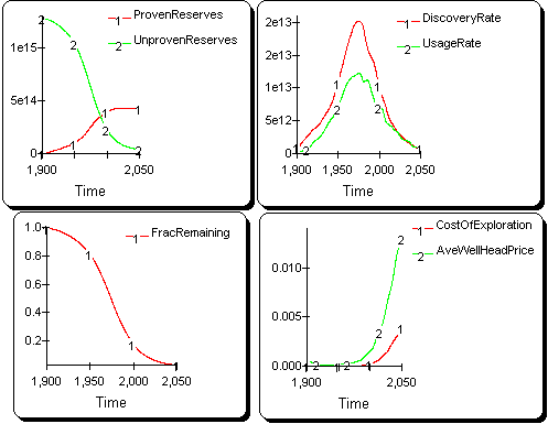
Figure 10: Time Series Plots from a Simulation of the Third Cut of Naill’s Model of U.S. Natural Gas Discovery and Production
Fourth Cut
Figures 11(a) and 11(b) illustrate the stock-flow and causal diagrams for the fourth step in the re-creation of Naill’s model of U.S. natural gas discovery and production. Figure 12 lists the corresponding equations for Figure 11(a) can be accessed by clicking directly on the diagram. The model has been extended through the addition of a balancing loop and a reinforcing feedback loop.
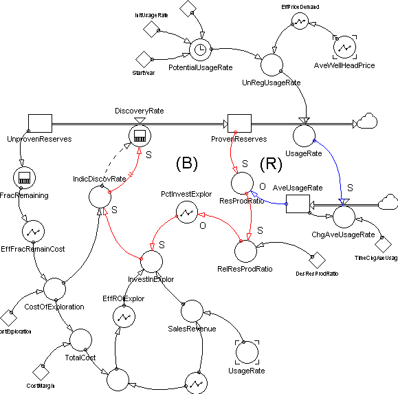
Figure 11(a): Fourth Cut of Naill’s Model of U.S. Natural Gas Discovery and Production.
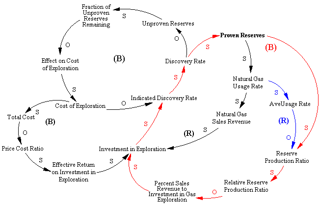
Figure 11(b): Causal Diagram of the Fourth Cut of Naill's Model of U.S. Natural Gas Discovery and Production.
The logic of the balancing loop (shown in red) is as follows. A rise in ProvenReserves, ceteris paribus, causes a rise in the reserve-production ratio (ResProdRatio), which is the number of years proven reserves will last, given the usage rate. A rise in the ResProdRatio, ceteris paribus, causes a rise in the relative reserve-production ratio (RelResProdRatio), which is a ratio of the reserve-production ratio to its desired value. A rise in the RelResProdRatio, ceteris paribus, causes a fall in the percent of sales revenue devoted to investment in gas exploration (PctInvestExplor). A fall in the PctInvestExplor, ceteris paribus, causes a fall in InvestInExplor. A fall in InvestInExplor, ceteris paribus, causes a fall in the IndicDiscovRate. A fall in the IndicDiscovRate, ceteris paribus, causes a fall in the DiscoveryRate which, after a significant delay, closes the loop and ensures, ceteris paribus, that proven reserves will be lower than they otherwise would have been. The logic of the reinforcing loop (shown partially in blue) is as follows. A rise in ProvenReserves, ceteris paribus, causes a rise in the natural gas usage rate (UsageRate). A rise in the UsageRate, ceteris paribus, causes a rise in the ChgAveUsageRate, which is a flow that changes the average usage rate (AveUsageRate). A rise in the ChgAveUsageRate, ceteris paribus, causes a rise in the AveUsageRate. A rise in the AveUsageRate, ceteris paribus, causes a fall in the ResProdRatio. A fall in the ResProdRatio, ceteris paribus, causes a fall in the RelResProdRatio. A fall in the RelResProdRatio, ceteris paribus, causes a rise in the percent of sales revenue devoted to investment in gas exploration (PctInvestExplor). A rise in the PctInvestExplor, ceteris paribus, causes a rise in InvestInExplor. A rise in InvestInExplor, ceteris paribus, causes a rise in the IndicDiscovRate. After a significant delay, a rise in the IndicDiscovRate, ceteris paribus, causes a rise in the DiscoveryRate, which closes the loop and ensures, ceteris paribus, that proven reserves will be higher than they otherwise would have been. Figure 13 shows time series plots from a simulation of the model presented in Figures 11. A comparison with Figure 10 reveals that the model now exhibits two new behaviors. The first is an oscillation that is most apparent in the plots of proven reserves, the discovery rate, and the usage rate. The second is that proven reserves now rise, peak and fall, instead of merely rising and peaking as in the last version of the model. The model’s oscillatory behavior can be readily explained. A rule of thumb in system dynamics modeling is that oscillation is caused by a balancing feedback loop with delayed corrective action. The balancing loop (negative feedback) that was added to this version of the model provides precisely this type of structure. That is, the model adjusts its investment in exploration by watching its reserve-production ratio. When proven reserves drop and the reserve-production ratio falls below its desired level, more revenue is invested in exploration. When proven reserves rise and the reserve-production ratio exceeds its desired level, investment in exploration falls. Because of the significant delay between the time a monetary investment in exploration is made and the time natural gas discoveries occur, by the time new proven reserves are added to ProvenReserves, they are no longer the amount necessary to bring the reserve-production ratio into line with its desired value. As a result, the model must again adjust its investment in exploration via the balancing loop. The system ends-up out of sync -- over and undershooting its desired reserve-production ratio.
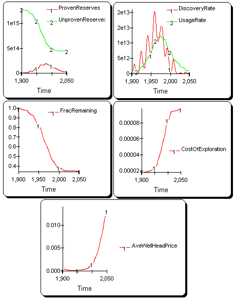
Figure 13: Time Series Plots from a Simulation of the Fourth Cut of
Naill’s Model of U.S. Natural Gas Discovery and Production
Fifth Cut
Figure 14(a) and 14(b) illustrate the fifth step in the recreation of Naill’s model of U.S. natural gas discovery and production. Figure 15 shows the equations corresponding to the simulation model. To view Figure 15, click directly on the stock-flow diagram. The main additions to the model are pieces of system dynamics structure that enable the system to determine the price of natural gas endogenously, rather than exogenously, as in past versions of the model. At present, this pricing structure assumes that natural gas prices are not regulated. The way that this constraint can be relaxed will be addressed in the next version of the model.
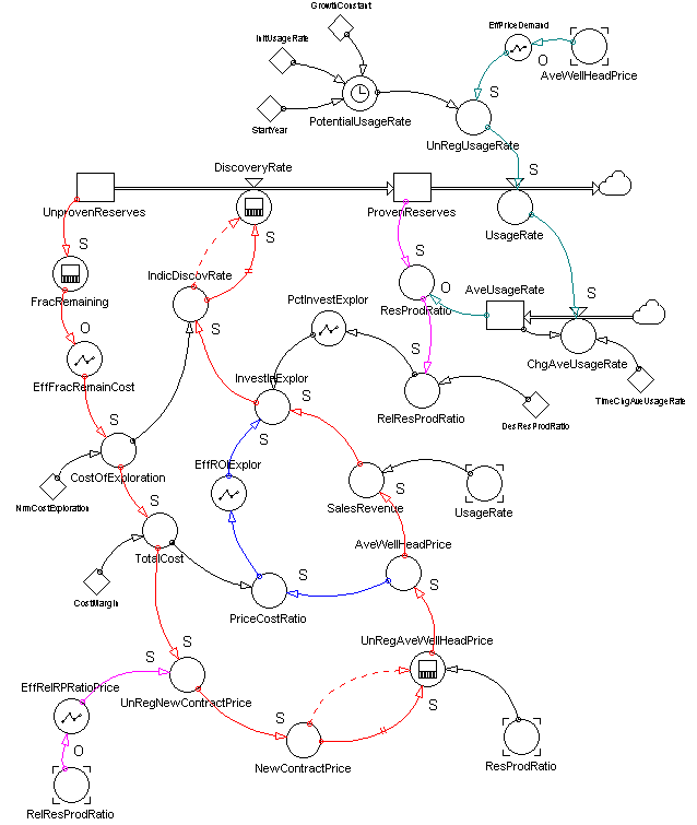
Figure 14(a): Fifth Cut of Naill's Model of U.S. Natural Gas Discovery and Production
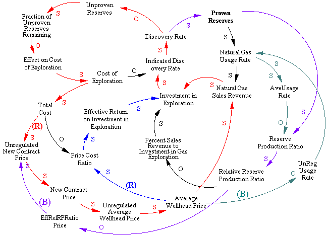
Figure 14(b): Causal Diagram of additional balancing and reinforcing loops for Cut 5 model.
The addition of an endogenous pricing structure creates four new feedback loops in the model. Two of the loops are reinforcing loops (positive feedback) and two are balancing loops (negative feedback). These loops can be identified in Figure 14, wholly or partially, via information links of different colors. The first new loop (shown with red information links) is a reinforcing loop. This loop works through gas price and hence sales revenue to keep gas discoveries rising as depletion occurs. The second new loop (shown partially in blue) is also a reinforcing loop. In a way similar to the previous loop, this loop works through gas price and return on investment in exploration to keep gas discoveries rising as depletion occurs. The third new loop is a balancing loop. It is shown partially in Figure 14 with purple information links. This loop works to keep the reserve-production ratio at its desired level by changing gas price and hence new gas discoveries. In other words, this loop represents the effects of gas price on the supply side of the gas system. The fourth new loop shown partially in Figure 14 with teal information links is also a balancing loop. This loop works to keep the reserve-production ratio at its desired level by changing gas price and hence the gas usage rate. In other words, this loop represents the effects of gas price on the demand side of the gas system. Figure 16 shows time series plots from a simulation of the model presented. A comparison with Figure 13 reveals that the model’s behavior is essentially the same as before, although its oscillations are less severe. This damping of the system’s oscillations, of course, is due to the feedback loops that were added to the system. Movements in the price (market) system take away some of the pressure on the system to change via the percent of revenues invested in gas exploration and discovery.
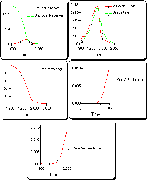
Figure 16: Time Series Plots from a Simulation of the Fifth Cut of Naill’s Model of U.S. Natural Gas Discovery and Production
Sixth Cut
Figure 17 illustrates the stock-flow diagram for the sixth step in the recreation of Naill’s model of U.S. natural gas discovery and production. To view equations that correspond to model (Figure 18), click direct on the stock-flow diagram. The main additions to the system are pieces of structure that enable a model user to easily change policies, such as gas price regulation, during the simulation run.
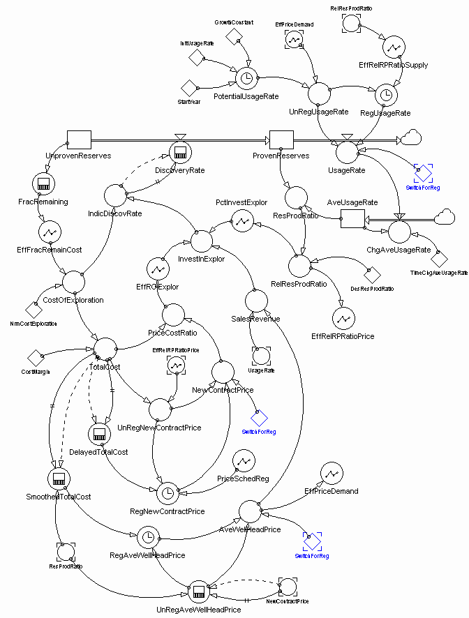
Figure 17: Sixth Cut of Naill's Model of U.S. Natural Gas Discovery and Production.
Price regulation is turned on in the model by changing a "switch" (SwitchForReg), shown in blue, from a zero to a one. When the switch is flipped, gas price is determined from both endogenous (TotalCost) and exogenous pressures (a price ceiling whose value is determined outside of the model (presumably by the government)). If, on the other hand, SwitchForReg remains set at zero, gas price is again determined endogenously via pressures from both TotalCost and the EffRelResProdRatio. Figure 19 shows time series plots from a simulation of the model with no price regulation. This run is directly comparable to previous model runs. When examined relative to Figure 16, it is clear that the model’s (unregulated) behavior has essentially not changed. On the other hand, Figure 20 shows time series plots from a simulation of the model under the assumption of price regulation during the years 1955-1980; the simulation is fairly similar to the one presented in Figure 19, although there is a large "blip" upward in the discovery rate, usage rate, and in proven reserves in 1980, when gas price deregulation occurs. Overall, however, the basic behavior mode of growth, peaking and decline has not changed.
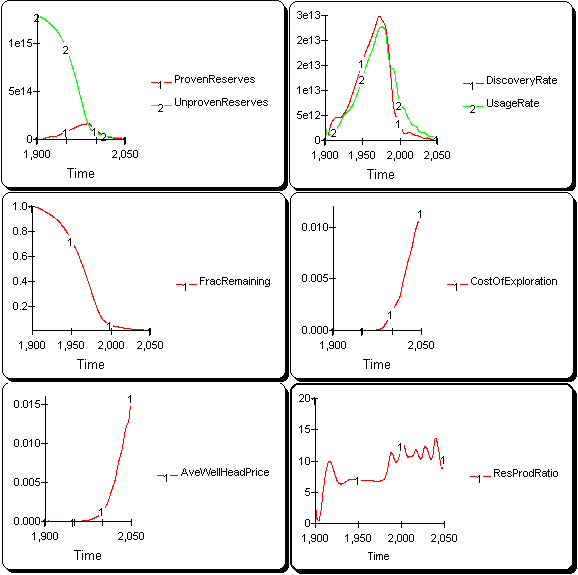
Figure 19: Time Series Plots from a Simulation of the Sixth Cut of Naill’s Model of U.S. Natural Gas Discovery and Production: Unregulated Scenario
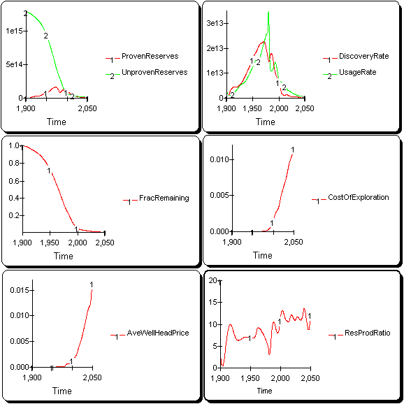
Figure 20: Time Series Plots from a Simulation of the Sixth Cut of Naill’s Model of U.S. Natural Gas Discovery and Production: Regulated Scenario
Finally, in the Reference Modes section of this chapter, we presented some actual data from the U.S. natural gas system including actual discovery rate, usage (production) rate, proven reserves, and reserve-production ratio. Although these data do not span the entire life cycle of the natural gas system (roughly the years 1900 to 2050) a la Hubbert, they were used to complement the reference modes resulting from Hubbert's theory and to calibrate the model. Figure 21 shows the time series plot comparing the actual data to simulated data between the years 1975 to 1995.
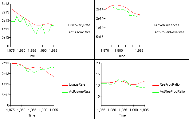
Figure 21: Time series plot comparing the actual data to simulated data between the years 1975 to 1995.
Policy Explorations with Natural Gas Model
Now that you have been introduced to the underlying assumptions of the system dynamics model for the natural gas industry, it is time to use the model to conduct your own policy experiments. The figure below illustrates the basic layout of the flight simulator version of the Natural Gas Discovery Model. To launch the "flight simulator" version of the Natural Gas Discovery model, click on the rotating icon . Then try some of the experiments suggested below. Once you have gained some familiarity with using the model, you can begin to develop your own experiments.
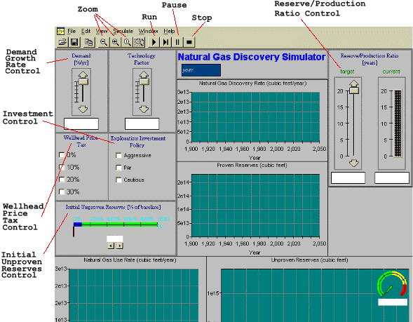
Figure 1:Layout of the Natural Gas Discovery Simulator
Establishing the base run
For these policy experiments, we first want to establish a base run. A base run is our first estimate of how we think the system works today. By establishing this as a baseline, we then can compare the results of each change in the model back to the base. Follow the steps listed below:
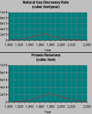
Figure 2: Example time series plot of base run Proven Reserves and Discovery Rate variables.
After checking through the different graphs, you should be ready to start changing parameters in the model to see how the simulation can unfold differently under different policies and scenarios. The control panel contains two kinds of parameters for you to control: Policy Levers and Uncertainties variables.
We will walk you through one experiment in more detail to illustrate the steps of changing the policy and explane the results, and then set you loose to experiment with the rest.
[Guided Experiment]
What if the unproven reserves of natural gas were 50% greater than we first estimated? This is an experiment in which we are going to alter one of the "uncertainties" in the model to see how much difference it will make in the behavior of the natural gas industry:
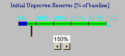
Figure 3: Setting initial uproven reserves to 50% greater than base case
One of the sets of graphs are called comparative graphs and allow the same variable to be shown on the same graph for multiple experiments, as shown in Figure 3 below:
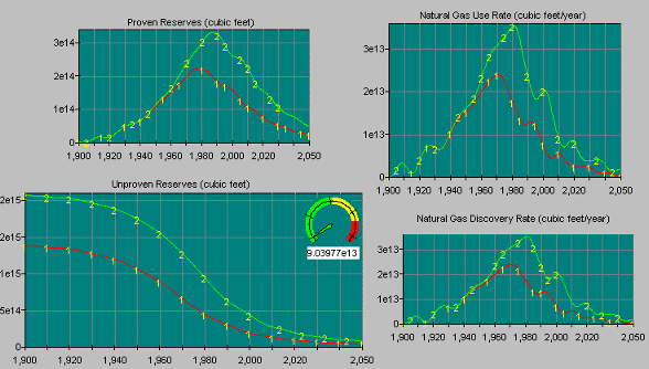
Figure 4: Comparison of base run and results of increasing base unproven reserves by 50%.
One of the sets of graphs are called comparative graphs and allow the same variable to be shown on the same graph for multiple experiments, as shown in Figure 3 below:
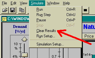
Figure 5: Clearing Experiment Results
Suggested Experiments
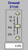 | Conservation policy 1- What would happen if the government (or industry) set up a policy to encourage the conservation of natural gas whenever the proven reserves fall? We can simulate this policy through the natural gas Demand variable in the control panel. This variable can be changed at any time during the simulation. |
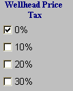 | Conservation policy 2 - Use a simple tax on the wellhead price to discourage use of natural gas. Use the Wellhead Price Tax box to tax. |
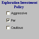 | Exploration Investment - What would happen if industry was more aggressive in their efforts to discover new sources of natural gas? We can model this policy by changing the base fraction of revenues invested in exploration. |
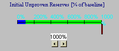 | Amount of unproven reserves - One of the fundamental uncertainties of natural resources is that we don't know how much is underground that we have not yet discovered. An important test of the natural gas system is to find out how much difference it would make if there were twice as much as we first estimated. What would happen if there were ten times (1000% of baseline) as much? |
 | Base usage growth rate - Another important uncertainty in the future of the natural gas industry is the growth rate of the demand for energy. This variable is the percent increase in the base demand for natural gas. |
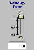 | Technology Investment - The technology multiplier is a multiplier against the cost of exploration. It represents advances in technology that make it cheaper to access the unproven natural gas. Change this multiplier to a fraction of the base cost to see the impact of a technology advance at any time during the simulation. |
[Previous] |
|
[Next] |
 |
Updated : 2005/07/23 |